
There are many scenarios you may come across while working in Excel where you only desire unique values in a list. You might want to rid your data of duplicates to create summaries, populate drop-down lists, or remove duplicates that found their way into your spreadsheet. Luckily, Microsoft Excel offers many ways to accomplish this, and depending on your particular situation, you may use different methods to accomplish the task at hand. In this article, we’ll cover a bunch of different ways to identify those unique values so you have a full set of tactics to handle anything thrown your way. Let’s dive in!
The UNIQUE Function
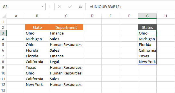
With the release of Dynamic Array functions in 2020 (M365 only), Excel now offers a powerful function right out of the box to provide a simple way to pull together a list of unique values. Simply input the range you would like to analyze inside the UNIQUE Function and you’ll have the unique results delivered in a Spill Range below the formula.
If you’re looking for a more long-term solution, convert your data set into an Excel Table (ctrl + t) and point your UNIQUE function to read the table column. This will allow you to always have a more dynamic listing as your data grows or shrinks over time.
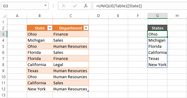
Pro Tip: If you want your list in alphabetical order add the Sort Function to your formula:
=SORT(UNIQUE(Table1[State]))
Array Formula
Before the UNIQUE function was released, Excel users were left using more complex methods to compile a list of unique values from a range. Pretty much all of these methods involved using array formulas (think Ctrl+Shift+Enter) to output the end result. The formula I will share in this post does not require keying in Ctrl+Shift+Enter to activate it, hence why I prefer it. The downside to using an Array formula over an Dynamic Array function is you have to carry it down manually, there is no Spill Range functionality that will automatically resize your list.
I won’t go into the details of how this formula works (if interested go here), just know if you set it up properly it will magically work. Make sure you pay close attention to your dollar signs at the beginning of the COUNTIF function. It does matter that the first cell reference stays static while the other one changes as you carry the formula down (ie $G$3:G3 in the below example).
Finally, after you setup the first formula, you’ll need to drag the formula down until you start seeing #N/As. You’ll want to monitor your list if your data will be changing in the future to ensure it is picking up all the unique results. As a rule, I always make note to ensure at least one #N/A is showing at the bottom of my list.
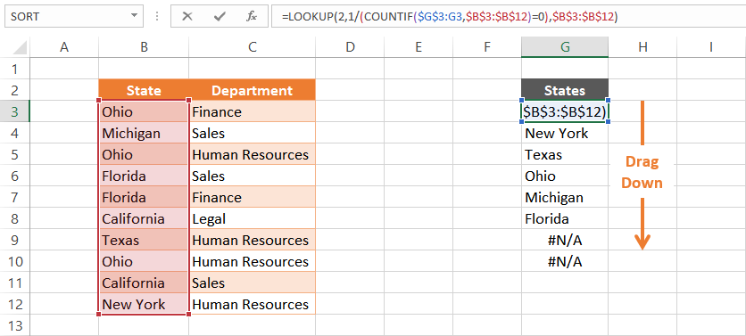
FORMULA: =LOOKUP(2,1/(COUNTIF($G$3:G3,$B$3:$B$12)=0),$B$3:$B$12)
Apply A Filter
If you would like to see a list of unique values without necessarily needing to store the list, you can utilize a cell Filter (ctrl + shift + L). Apply a filter to your data and click the filter arrow to see a list showing all the unique values within that particular column of data.

Pivot Table
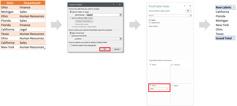
A Pivot Table is another good way to list out unique values. Select your data range (ensuring every column has a unique header value) and go to Insert > Pivot Table. When the Insert Dialog box appears , simply hit the OK button and you can start pivoting your data.
click to enlarge
Drag the name of the column you would like to see a unique list of value for into the “Rows” quadrant. You should instantly see your list populate within the Pivot Table.
Remove Duplicates
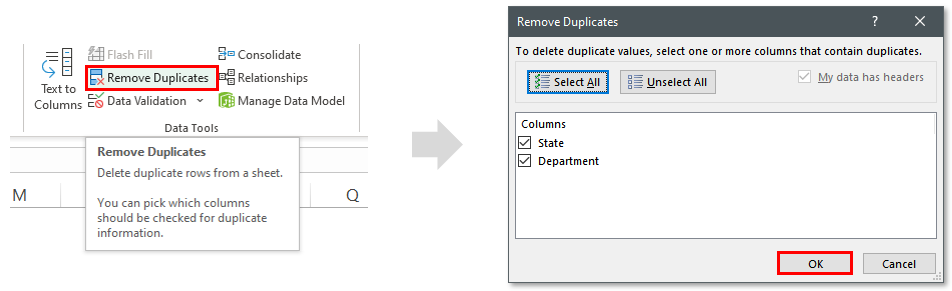
If you actually want to modify your data so it only has unique values, you can utilize Excel’s Remove Duplicate button. This feature can be used on a range of cells or within an Excel Table.
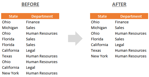
Follow these steps to utilize this functionality:
Select your range of data
Navigate to the Data Ribbon tab.
Click the Remove Duplicates button within the Data Tools button group
Check the combination of columns you’d like to be unique
Highlight Duplicates
If you are wanting to ensure your spreadsheet is constantly checking for instances where duplicates might slip-in, there are a couple of methods you can integrate into your worksheet:
Conditional Formatting
You may run into situations where you want to quickly visualize if there are any duplicates in your data set. This is where you can apply a little bit of conditional formatting and luckily there is a preset to flag duplicate values!
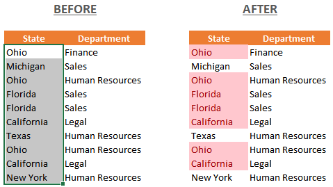
Just follow these simple steps:
Highlight the cell range you want to analyze
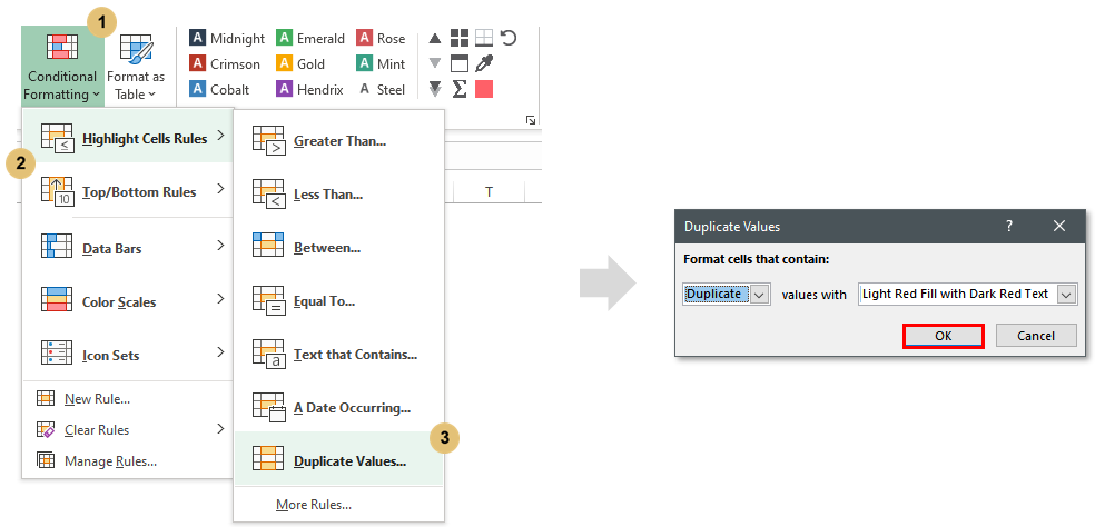
Navigate to the Conditional Formatting button on the Home tab
Select Highlight Cells Rules
Select Duplicate Values…
Click OK
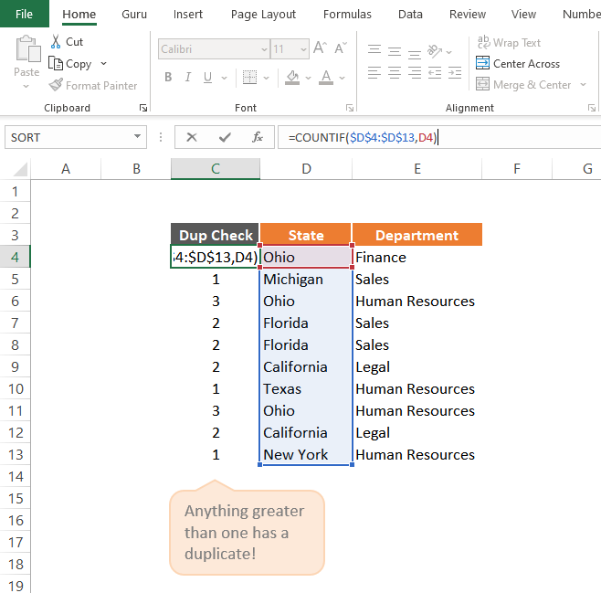
Counting Formula
You might want to pursue utilizing a formula to flag your duplicate values. This can be done by using the COUNTIF() function. The below example shows how you can analyze each cell in the data range and understand if that value occurs more than once. If you have any count that is great than 1, you know there’s a duplicate within your data set.
Example Formula: =COUNTIF($D$4:$D$13, D4)
After you have implemented the formula, simply apply a filter and filter out all the “1” values.
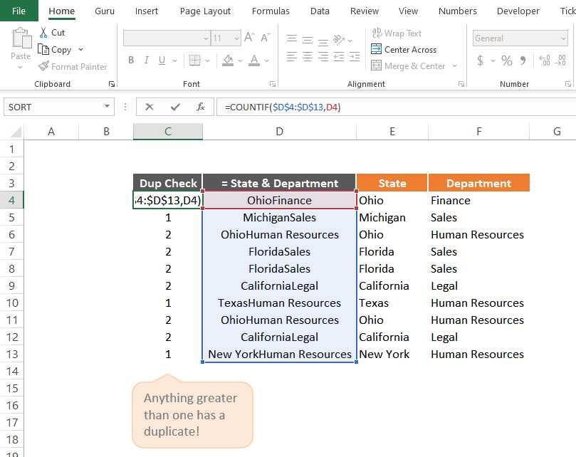
If you are more concerned with having a duplicate row across multiple columns, you can add a helper column (Column D in the below example) that joins the values of the columns you want to ensure are unique. After the helper column is created, point your COUNTIF function to it and repeat the steps in the prior example.
Any Others I Missed?
Whew, that was a lot of techniques we went through to get to pretty much the same result. Hopefully, you start to realize as you find yourself needing to pull together a list of unique values, how valuable knowing all the options available to you in Excel. I’m sure there were other great methods that I overlooked or haven’t discovered yet. Please let me know if you have any tips in the comments section and I can growth this article even further!
I Hope This Helped!
Hopefully, I was able to explain how you can use a variety of methods to create unique lists of your data. If you have any questions about this technique or suggestions on how to improve it, please let me know in the comments section below.

About The Author
Hey there! I’m Chris and I run TheSpreadsheetGuru website in my spare time. By day, I’m actually a finance professional who relies on Microsoft Excel quite heavily in the corporate world. I love taking the things I learn in the “real world” and sharing them with everyone here on this site so that you too can become a spreadsheet guru at your company.
Through my years in the corporate world, I’ve been able to pick up on opportunities to make working with Excel better and have built a variety of Excel add-ins, from inserting tickmark symbols to automating copy/pasting from Excel to PowerPoint. If you’d like to keep up to date with the latest Excel news and directly get emailed the most meaningful Excel tips I’ve learned over the years, you can sign up for my free newsletters. I hope I was able to provide you some value today and hope to see you back here soon! - Chris